This simulation was the final project in my computer engineering applications (ie, Matlab) class. I was just following an algorithm and some initial conditions provided so I really don't know anything about the oil spill itself or if this is an accurate simulation, but I think it demonstrates a couple of useful techniques for graph generation & visualization. Please see the Source Code (GPL License)

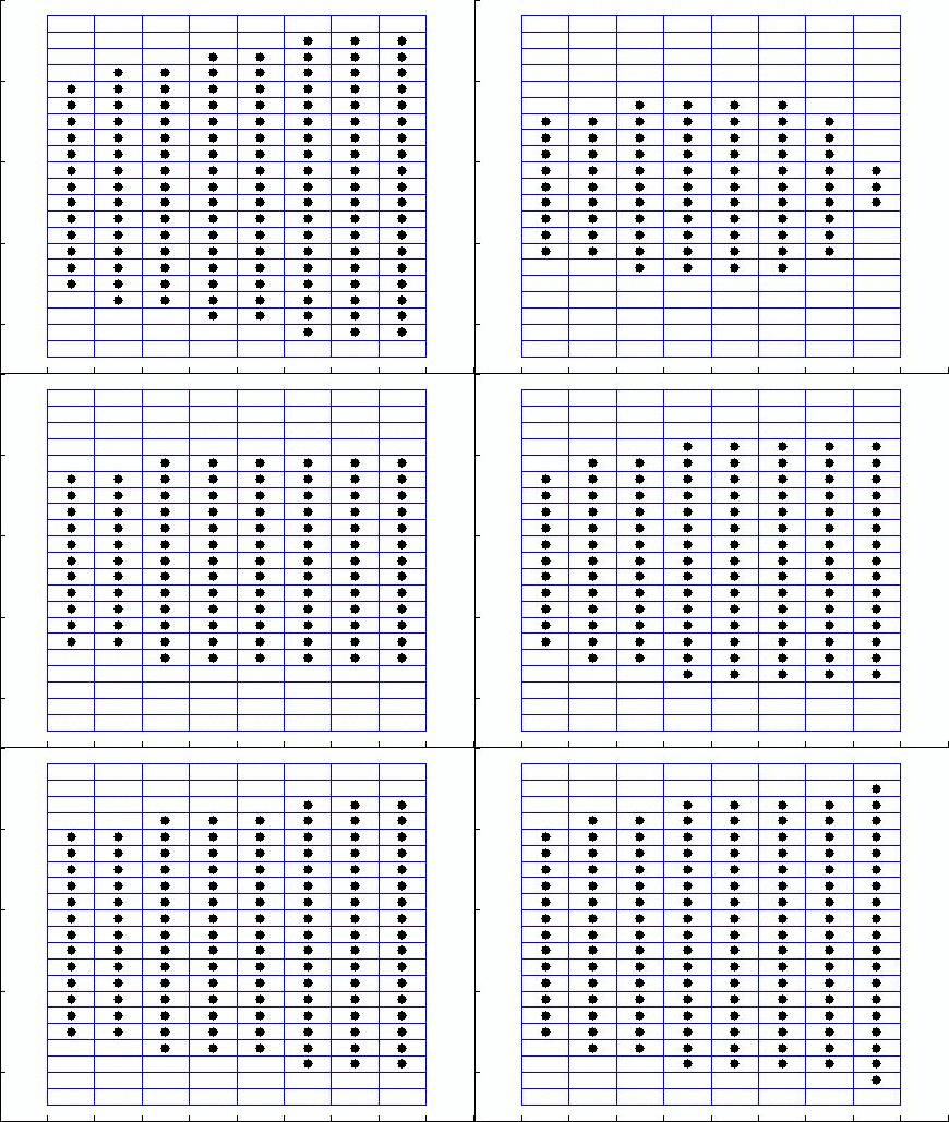
Result of Default Parameters:

This image shows the oil spill stemming from the center-left of the grid. The oil spreads almost immediately into the east, but the number of captures is set too low to see any cells become oil-free.

Capturing Simulation into a Movie

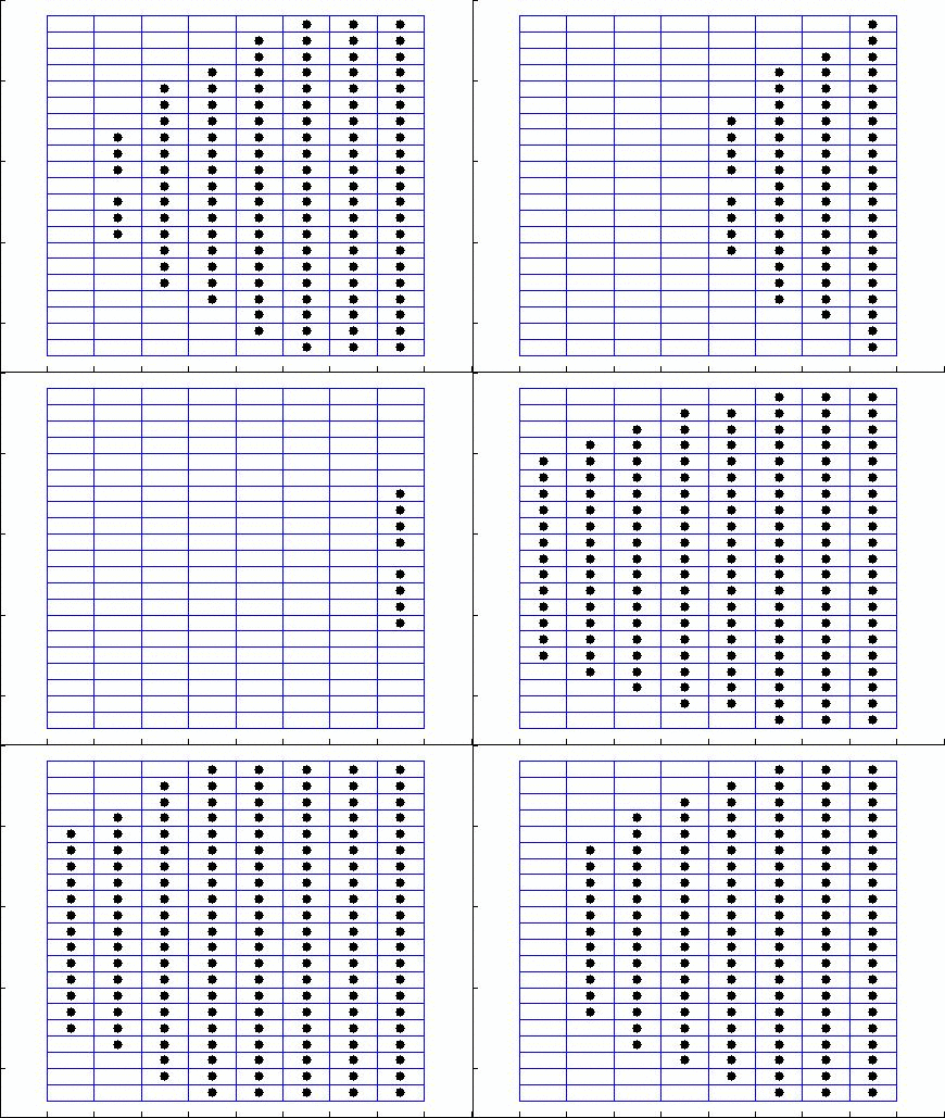
Matlab provides the very convenient movie() function, enabling visualizations of graph changes over time. This simulation uses a grid-overlayed scatterplot to show oil propagation and ties a number of these state captures together.

None of the default visualizations are really intended for spatial data. Conveniently, the simulation already works on a grid; After drawing a grid for each frame, the mapping from array data to spatial data is apparent.

I really wanted to use such toys as the Google Earth toolbox or the Google Maps loader to overlay the simulation grid on top of the real location in the Prince William Sound. I decided against it only because of the unknown accuracy of the simulation; It seemed a little pointless since I don't actually know which way the wind really blows.

Saving/Loading Figures

Drawing a grid is actually a rather painful process, and attempting to do so on-the-fly would make the runtime unreasonable.

This script generates and saves a grid figure to serve as the field, then uses load(file, '-mat') to load the figure. I elected to use load instead of hgload in order to avoid opening the figure while drawing. Ironically, after going through all the effort of 'silently' drawing each frame, I discovered that movie() forces a frame to become visible briefly in order to capture it.

load(file, '-mat') loads the figure data into a matlab structure; The relevant figure data (a nested structure) is hiding inside of the hgS_070000 key. This is then converted into a figure with struct2handle(figure.hgS_070000, 0) -- the zero corresponding to the parent figure. ('root figure': the Matlab environment.)

Usage & Limitations:

• Script was created and tested on R2011A. I have no idea about other versions, but it should work.
• You cannot execute this script using cell mode because it doesn't set the PATH correctly.
• If you find yourself playing with the parameters a lot, you might want to check out the console simulation mode. It skips the lengthy generation of images for the 'movie' and just prints out the current state on the console.

Parameter Notes:

• Gallons Spilled: The maximum value, 100k, is still 110 times smaller than the accepted estimate for the real spill.
• Wind Velocity: Any value of significance quickly blows the oil out of the field; Wind speeds can reach as high as 40 miles per hour, which yields depressing results.
• Iterations: More captures will make not only for a richer simulation, but also a longer one. Too long of a simulation and you may be watching the open ocean for a while. (And waiting a long time to watch anything.)

Result of Higher Parameters:

With evaporation and wind velocity set to higher values, oil can be seen being blown out/evaporated out of cells. Most of the oil is just being blown around, though, probably mostly onto Bligh Island. (Directly to the east of the spill location. )